# Adding and managing content
This section of the Guide describes the various tools and approaches available to catalog administrators to add, edit, organize, and delete catalog entries (datasets).
# Data types and external resources
NADA distinguishes entries by data type. For each data type, a specific metadata standard or schema must be used to generate and store the metadata. The information contained in the metadata, and the way the metadata will be displayed and made searchable and accessible, is thus specific to each data type. Instructions are thus provided for each type of data, although the core principles are the same for all types of data. Also, external resources (which you can interpret as "any related electronic file that should be provided in a catalog entry page") can be attached to catalog entries independently of the data type.
# Data types
As a reminder, the data types that NADA can ingest, and the related metadata standards and schemas, are the following:
Microdata: Microdata are the unit-level data on a population of individuals, households, dwellings, facilities, establishments, or other. They can be generated from surveys, censuses, administrative recording systems, or sensors. Microdata are documented using the DDI-Codebook metadata standard.
Statistical tables: Statistical tables are summary (aggregated) statistical information provided in the form of cross-tabulations, e.g., in statistics yearbooks or census reports. They will often be a derived product of microdata. Statistical tables are documented using a metadata schema developed by the World Bank Data Group.
Indicators and time series: Indicators are summary (or aggregated) measures derived from observed facts (often from microdata). When repeated over time at a regular frequency, the indicators form a time series. Indicators and time series are documented using a metadata schema developed by the World Bank Data Group.
Geographic datasets and geographic data services: Geographic (or geospatial) data identify and depict geographic locations, boundaries, and characteristics of the surface of the earth. They can be provided in the form of datasets or data services (web applications). Geographic datasets and data services are documented using the ISO 19139 metadata standard.
Documents: Text is data. Using natural language processing (NLP) techniques, documents (i.e. any bibliographic citation, such as a book, a paper, and article, a manual, etc.) can be converted into structured information. NLP tools and models like named entity recognition, topic modeling, word embeddings, sentiment analysis, text summarization, and others make it possible to extract quantitative information from unstructured textual input. Documents are documented using a schema based on the Dublin Core with a few aditional elements inspired by the MARC21 standard.
Images: This refers to photos or images available in electronic format. Images can be processed using machine learning algorithms (for purposes of classification or other). Note that satellite or remote sensing imagery are considered here as geographic (raster) data, not as images. Images are documented using either the IPTC metadata standard, or the Dublin Core standard.
Videos. Videos are documented using a metadata schema inspired by the Dublin Core and the VideoObject schema from schema.org (opens new window).
Scripts: Although they are not data per se, we also consider the programs and scripts used to edit, transform, tabulate, analyze and visualize data as resources that need to be documented, catalogued, and disseminated in data catalogs. Scripts are documented using a metadata schema developed by the World Bank Data Group.
Information on the metadata standard and schemas is available at https://ihsn.github.io/nada-api-redoc/catalog-admin/# (opens new window) and in a Schema Guide.
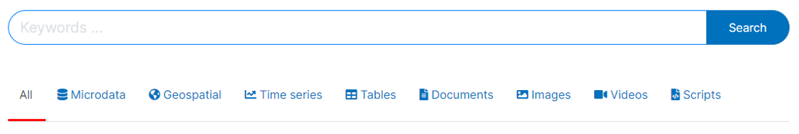
# Data type tabs
In the NADA catalog, data will be organized by type. ALL entries are listed in the first tab, labeled "All". The entries for each data type will be displayed in a separate tab in the catalog listing. This will allow users to focus their attention to data of the type of interest.
NADA will only display a tab when there is at least one data of the corresponding type in the catalog. Tabs are automatically added when an entry for a new data type is added.
The sequence in which the tabs are displayed can be controlled.
@@@@@@@@@
# External resources
External resources are electronic files (or links to electronic files) of any type, that you may want to attach to an entry metadata as "related materials". This could for example be the PDF version of the survey questionnaire and interviewer manual related to a survey microdataset, or visualizations related to a published document. A simple metadata schema (based on the Dublin Core standard) is used to document external resources. This schema includes an element that indicates the type of the resource (e.g., microdata, analytical document, administrative document, technical document, map, website, etc.) In NADA, you will publish the metadata related to a dataset, then add such external resources to it.
# Adding a catalog entry: four approaches
A new entry can be added to a NADA catalog in different manners. We already mentioned that this can be done either using the web interface, or using the catalog API and a programming language.
The way an entry is added to a NADA catalog will also depends on the form in which the metadata are available:
- When metadata compliant with one of the recognized standards and schemas is provided in electronic files: the process will then consist of uploading the metadata file(s), uploading the related resource files (data, documents, etc.), and selecting data dissemination options (access policy). Uploading such files can be done using the web interface or using the API.
- When metadata are not readily available in an electronic file, metadata can be created from scratch in NADA and published using the web interface. This option is not (yet) available for Geospatial data, and is not recommended for microdata.
- When metadata are not readily available in an electronic file, metadata can be created using a programming language (R or Python) and published using the API.
We briefly present these three options below. In subsequent sections, we will describe in detail how they are applied (when available) to each data type.
# Loading metadata files using the web interface
When metadata files compliant with a metadata standard or schema recognized by NADA are available (typically generated using a specialized metadata editor), these files can be uploaded in NADA using the web interface. The interface will also be used to upload the related resource files (the external resources), to add a logo/thumbnail, and to specify the dataset access policy. This approach currently applies only to microdata and external resources. It will be added to other data types in future releases of NADA.
To use this approach, you will need to access the page in the administrator interface where you can add, edit, and delete entries.
Click on Studies > Manage studies and select the collection in which you want to add an entry (if you have not created collections, the only option will be the Central Data Catalog).
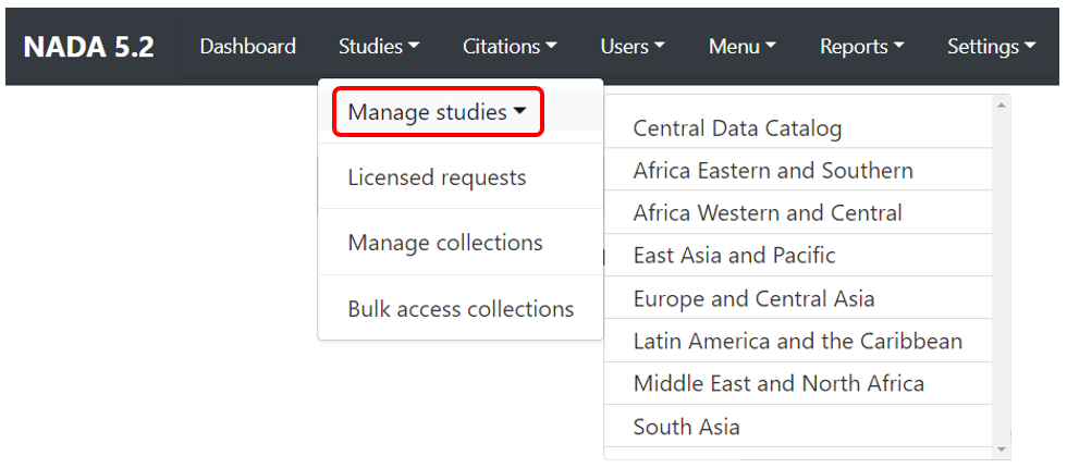
A list of entries previously entered in the catalog/collection will be displayed, with options to search and filter them.
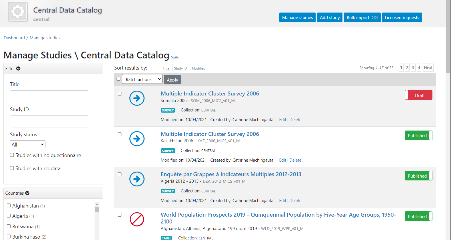
In this page, the Add study button will allow you to access the pages where entries can be added.

# Creating an entry from scratch using the web interface
The metadata can be created directly in NADA, using the embedded metadata editor. This approach will also require access to the "Add entry" page of the NADA administrator interface (see above). The option is available for all data types but is recommended only for data that require limited metadata (such as images, or documents). For other types of data, manually generating comprehensive metadata can be a very tedious process (e.g., for microdata where metadata related to hundreds if not thousands of variables would have to be manually entered).
# Loading metadata files using the API
This approach currently applies only to microdata, geographic datasets, and external resources. It will be added to other data types in future releases of NADA.
If you use this approach, you will need an API key with administrator privileges. API keys must be kept strictly confidential. Avoid entering them in clear in your scripts, as you may accidentally reveal your API key when sharing your scripts (if that happens, immediately cancel your key, and issue a new one).
Once you have obtained a key (issued by a NADA administrator), you will have to enter it (and the URL of the catalog you are administering) before you implement any of the catalog administration functions available in NADAR or PyNADA. This will be the first commands in your R or Python scripts. It is done as follows:
Using R:
library(nadar)

my_key <- read.csv("*...*/my_keys.csv", header=F, stringsAsFactors=F)
set_api_key(my_key\[5,1\]) # Assuming the key is in cell A5
set_api_url("http://*your_catalog_url*/index.php/api/")
set_api_verbose(FALSE)
Using Python:
import pynada as nada
my_key = pd.read_csv(".../my_keys.csv", header=None)
nada.set_api_key(my_keys.iat\[4, 0\])
nada.set_api_url(\'https:// *your_catalog_url* /index.php/api/\')
Then use function in NADAR or PyNADA to add an entry by importing the metadata using the available import functions. In NADAR: - import_ddi - geospatial_import - external_resources_import
Examples are provided in the next sections.
# Creating an entry from scratch using the API
Metadata can also be generated and published programmatically, for example using R or Python, and uploaded to NADA using the API and the NADAR package of PyNADA library. This option allows automation of many tasks and offers the additional advantage of transparency and replicability. For administrators with knowledge of R and/or Python, this is a recommended approach except for microdata (for which the best approach is to use a specialized metadata editor).
The metadata generated programmatically must comply with one of the metadata standards and schemas used by NADA, documented in the NADA API and in the Guide on the Use of Metadata Schemas. If you use this approach, you will need to provide an API key with administrator privileges and the catalog URL in your script, as shown in the previous paragraph. Then you add the code that generates the metadata and publish it in your catalog using the relevant _add function.
Metadata standards and schemas
The documentation of the metadata standards and schemas recognized by NADA is available at https://ihsn.github.io/nada-api-redoc/catalog-admin/# (opens new window). A Schema Guide is also available, which provides more detailed information on the structure, content, and use of the metadata standards and schemas.
In all schemas, most elements are optional. This means that schema-compliant metadata can be very brief and simple. Almost no one will ever make use of all metadata elements available in a schema to document a datatset. We provide below a very simple example of the use of R and Python for publishing a document (with only a few metadata elements).
# Generating compliant metadata using R
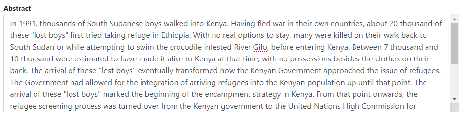
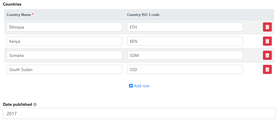
Metadata compliant with a standard/schema can be generated using R, and directly uploaded in a NADA catalog without having to be saved as a JSON file. An object must be created in the R script that contains metadata compliant with the JSON schema. The example below shows how such an object is created and published in a NADA catalog. We assume here that we have a document with the following information:
- document unique id: ABC123
- title: Teaching in Lao PDR
- authors: Luis Benveniste, Jeffery Marshall, Lucrecia Santibañez (World Bank)
- date published: 2007
- countries: Lao PDR.
- The document is available from the World Bank Open knowledge Repository at http://hdl.handle.net/10986/7710 (opens new window).
We will use the DOCUMENT schema to document the publication, and the EXTERNAL RESOURCE schema to publish a link to the document.
In R or Python, publishing metadata (and data) in a NADA catalog requires that we first identify the on-line catalog where the metadata will be published (by providing its URL) and provide a key to authenticate as a catalog administrator. We then create an object (a list in R, or a dictionary in Python) that we will name my_doc (this is a user-defined name, not an imposed name). Within this list (dictionary), we will enter all metadata elements, some of which can be simple elements, while others are lists (dictionaries). The first element to be included is the document_description, which is required. Within it, we add the title_statement which is also required and contains the mandatory elements idno and title (all documents must have a unique ID number for cataloguing purpose, and a title). The list of countries that the document covers is a repeatable element, i.e. a list of lists (although we only have one country in this case). Information on the authors is also a repeatable element, allowing us to capture the information on the three co-authors individually. This my_doc object is then published in a NADA catalog. Last, we publish (as an external resource) a link to the file, with only basic information. We do not need to document this resource in detail, as it corresponds to the metadata provided in my_doc. If we had a different external resource (for example an Excel table that contains all tables shown in the publication), we would make use of more of the external resources metadata elements to document it. Note that instead of a URL, we could have provided a path to an electronic file (e.g., to the PDF document), in which case the file would be uploaded to the web server and made available directly from the on-line catalog. We had previously captured a screenshot of the cover page of the document to be used as thumbnail in the catalog (optional).
library(nadar)

# Define the NADA catalog URL and provide an API key
set_api_url("http://nada-demo.ihsn.org/index.php/api/")
set_api_key("a1b2c3d4e5")  # Note: an API key must always be kept confidential

thumb  <- "C:/DOCS/teaching_lao.JPG"  # Cover page image to be used as thumbnail

# Generate and publish the metadata on the publication

doc_id <- "ABC001"

my_doc <- list(

   document_description = list(

      title_statement = list(
        idno = doc_id,
        title = "Teaching in Lao PDR"
      ),

      date_published = "2007",

      ref_country = list(
        list(name = "Lao PDR",  code = "LAO")
      ),

      # Authors: we only have one author, but this is a list of lists
      # as the 'authors' element is a repeatable element in the schema
      authors = list(
        list(first_name = "Luis",     last_name = "Benveniste", affiliation = "World Bank"),
        list(first_name = "Jeffery",  last_name = "Marshall",   affiliation = "World Bank"),
        list(first_name = "Lucrecia", last_name = "Santibañez", affiliation = "World Bank")
      )

   )

)

# Publish the metadata in the central catalog
add_document(idno = doc_id,
             metadata = my_doc,
             repositoryid = "central",
             published = 1,
             thumbnail = thumb,
             overwrite = "yes")

# Add a link as an external resource of type document/analytical (doc/anl).
external_resources_add(
  title = "A comparison of the poverty profiles of Chad and Niger, 2020",
  idno = doc_id,
  dctype = "doc/anl",
  file_path = "http://hdl.handle.net/10986/7710",
  overwrite = "yes"
)
The document is now available in the NADA catalog.
# Generating compliant metadata using Python @@@@
The Python equivalent of the R example provided above is as follows:
# Define the NADA catalog URL and provide an API key
set_api_url("http://nada-demo.ihsn.org/index.php/api/")
set_api_key("a1b2c3d4e5")  # Note: an API key must always be kept confidential

thumb  <- "C:/DOCS/teaching_lao.JPG"  # Cover page image to be used as thumbnail

# Generate and publish the metadata on the publication

@@@ doc_id = "ABC001"

document_description = {

  'title_statement': {
      'idno': "ABC001",
      'title': "Teaching in Lao PDR"
  },

  'date_published': "2007",

  'ref_country': [
		{'name': "Lao PDR", 'code': "Lao"}
	],

  # Authors: we only have one author, but this is a list of lists
  # as the 'authors' element is a repeatable element in the schema
  'authors': [
      {'first_name': "Luis",     'last_name': "Benveniste", 'affiliation' = "World Bank"},
      {'first_name': "Jeffery",  'last_name': "Marshall",   'affiliation' = "World Bank"},
      {'first_name': "Lucrecia", 'last_name': "Santibañez", 'affiliation' = "World Bank"},
  ]

}
Examples specific to each data type are provided in the next sections.
# Adding microdata

Creating a Microdata entry can be done in two different ways using the administrator interface and the API:
- By uploading pre-existing metadata (typically generated using a specialized metadata editor, like the Nesstar Publisher application for microdata) via the web interface.
- By generating and uploading new metadata using the web interface (but with limited capability to document variables; this is thus not a recommended option).
- By uploading pre-existing metadata (typically generated using a specialized metadata editor, like the Nesstar Publisher application for microdata) using the API.
- By generating and uploading new metadata programatically, using R or Python and the API.
Metadata standard: the DDI Codebook
For microdatasets, NADA makes use of the DDI Codebook (or DDI 2.n) metadata standard.
The documentation of the DDI Codebook metadata standards is available at https://ihsn.github.io/nada-api-redoc/catalog-admin/#tag/Survey (opens new window). A Schema Guide is also available, which provides more detailed information on the structure, content, and use of the metadata standards and schemas.
For microdata, the use of a specialized DDI metadata editor to generate metadata is highly recommended (like the Nesstar Publisher or the World Bank's Metadata Editor). Indeed, the DDI should contain a description of the variables included in the data files, preferably with summary statistics. Generating variable-level metadata can be a very tedious process as some datasets may include hundreds, even thousands of variables. Metadata editors have the capacity to extract the list of variables and some metadata (variable names, labels, value labels, and summary statistics) directly from the data files. The alternatives to generating the metadata using a specialized editor are to enter the metadata in NADA, or to enter them in R or Python scripts.
# Loading metadata (web interface)
If you have used a specialized metadata editor like the Nesstar Publisher software application to document your microdata, you have obtained as an output an XML file that contains the study metadata (compliant with the DDI Codebook metadata standard), and a RDF file containing a description of the related resources (questionnaires, reports, technical documents, data files, etc.) These two files can be uploaded in NADA.
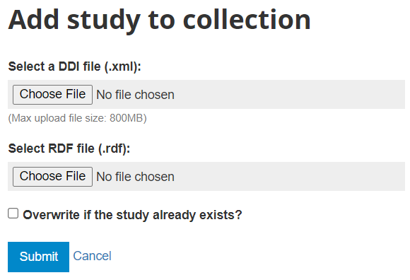
In the administrator interface, select Studies > Manage studies and the collection in which you want to add the dataset (if you have not created any collection, the only option will be to upload the dataset in the Central catalog; this can be transferred to another collection later if necessary). Then click on Add study.

In the Select a DDI file and Select RDF file, select the relevant files. Select the "Overwrite if the study already exists" option if you want to replace metadata that may have been previously entered for that same study. A study will be considered the same if the unique identification number provided in the DDI metadata field "study_desc > title statement > idno" is the same (in the user and administrator interface, IDNO will be labeled "Reference No"). Then click Submit.
The metadata will be uploaded, and an Overview tab will be displayed, providing you with the possibility to take various actions.
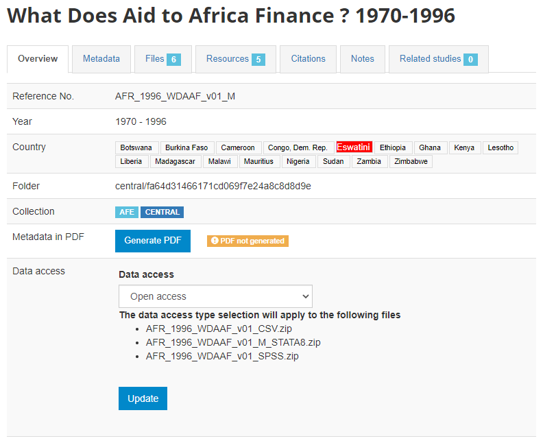
In Country, the names that are not compliant with the reference list of countries will be highlighted in red. By clicking on any of these country names, you will open the page where the mapping of these non-compliant names to a compliant name can be done. This is optional, but highly recommended to ensure that the filter by country (facet) shown in the user interface will operate in the best possible manner. See section "Catalog administration > Countries".
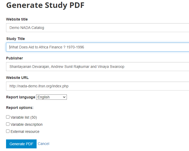
Metadata in PDF: Allows you to generate a PDF version of the metadata (applies to microdata only).

Data access: This is where you will indicate the access policy for microdata. The restrictions associated with some of these access policies will apply to all files declared as "Data files" in NADA (see description of tabs "Files" and "Resources" below. NADA must be informed of what files are "Data files"; it is very important when you document and upload external resources to make sure that data files are properly identified. If a data file is uploaded as a "document" for example, it will be accessible to users no matter the access policy you apply to the dataset.
The options for Data access are:
Open data: visitors to your catalog will be able to download and use the data almost without any restriction
Direct access: visitors will be able to download the data without restriction, but the use of the data is subject to some (minor) conditions
***Public Use Files (PUF)***: all registered visitors will be able to download the files after login; they will be asked but not forced to provide a description of the intended use.
Licensed data: registered visitors will be able to submit a request for access to the data by filling out an on-line form, which will be reviewed by the catalog administrator who can approve, deny, or request more information (see section "Managing data requests").
Data accessible in external repository: this is the option you will select when you want to publish metadata in your catalog but provide a link to an external repository where users will be able to download or request access to the data.
Data enclave: in this option, information is provided to users on how to access the data in a data enclave.
Data not accessible: in some cases, you will want to publish metadata and some related resources (report, questionnaire, technical documents, and others) but not the data.
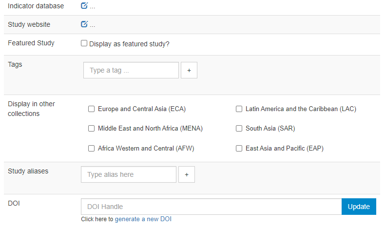
Indicator database: this applies to microdata only. The field allows administrators to provide the URL of a website were indicators generated out of the microdata are published.
Study website: a link to an external website dedicated to the survey.
Featured study: This allows administrators to mark entries as "featured". Featured studies will be shown on top of the list of entries in NADA catalogs, with a "Featured" pill.
Tags: Enter tags (each one with an optional tag group; tag groups will typically be used for creating custom facets; see section on Adding facets).
Display in other collections: The list of collections (if any) created in the catalog will be displayed. You can select the collections (other than the one in which you are publishing the dataset) in which you want your dataset to be visible. These collections will show but not own the dataset.
Study aliases: This field can be used to enter alternative names by which the dataset may be referred to.
DOI: The system allows administrators to request the issuance of a DOI for the dataset.
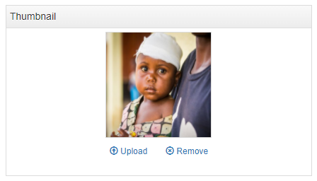
An image file can be selected to be used as thumbnail in the catalog. This thumbnail will be visible in the catalog listing page, and in the banner of the dataset page.
By default, the metadata you just published will be in draft mode in your catalog, i.e. not visible to users. To make the metadata visible in your catalog, click on "Draft" to convert the status to "Published". You can at any time unpublish a dataset; it will then become invisible to users, but will not be deleted from your catalog.

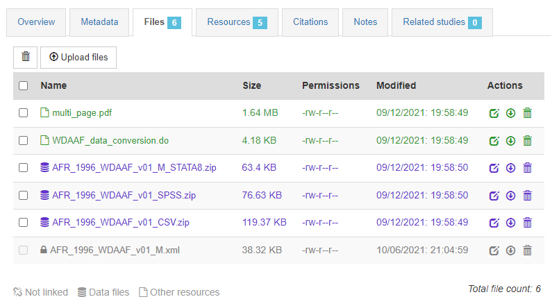
In the Files tab, you have the option to upload the files (data files or external resources) that you want users to be able to access from the online catalog. Some files have already been uploaded (the XML and RDF files); others will have to be manually uploaded to the web server.
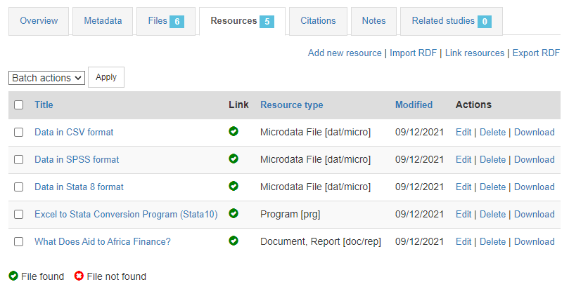
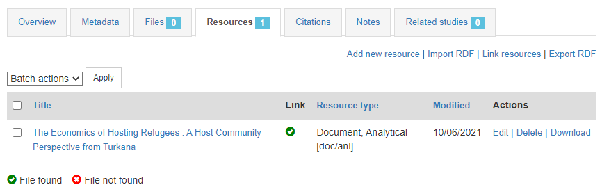
In the Resources tab, you will see a list of external resources, which should correspond to the files you uploaded. A green icon should appear next to the "Link", indicating that a file has indeed been identified that corresponds to the resource. If you see a red icon, click on "Link resources" to try and fix the issue. If the problem persists, the filename identified in the RDF metadata probably does not match the name of the uploaded file, or the file has not been uploaded yet (see Files tab).
That's it. Your data and metadata are now visible to all users who have access to your catalog.
# From scratch (web interface)
If you want to add a microdata entry to your catalog using the web interface, but do not have metadata ready to be uploaded (in the form of a DDI-compliant XML file and an optional RDF file), you have the possibility to create a new entry in the NADA administrator web interface. Note however that this option is limited to the study description section of the DDI metadata standard. The study description of the DDI standard describes the overall aspects of the study (typically a survey). Other sections of the DDI are used to document each data file (file description), and each variable (variable description). In the current version of the metadata editor embedded in the NADA web interface, the file and variable description sections are not included. For that reason, the use of this option is not recommended except for cases when no file and variable description is available. In other cases, the use of a specialized metadata editor (like the Nesstar Publisher) or the more complex programatic option (described below) are recommended. Documenting files and variables (when available) adds rich metadata that will increase the visibility, discoverability, and usability of your datasets.
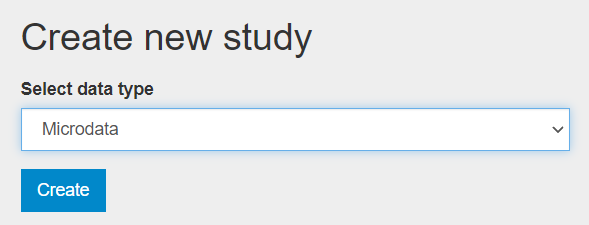
To document a micro-dataset from scratch using the web interface, select "Add study" in the dashboard page, then select the option microdata in the Create new study box. Then click Create.
The Overview tab of a new, empty entry will be displayed.
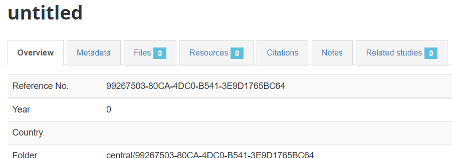
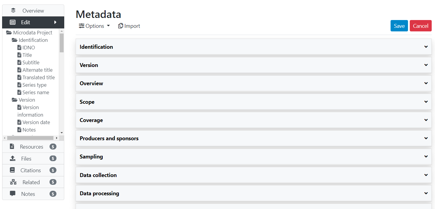
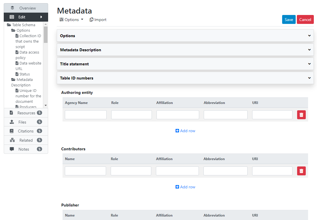
Click on the Metadata tab to open the (limited) DDI metadata editor. The left navigation bar allows you to navigate in the metadata entry form. Enter a much information as you can in the metadata fields, then click Save.

Once you have entered and saved metadata, proceed as explained in the previous section to upload files, select options, add a thumbnail, and publish your metadata. To add external resources, use the Add resource in the External resources page.
# Loading metadata (API)
If you have used a specialized metadata editor like the Nesstar Publisher software application to document your microdata, you have obtained as an output an XML file that contains the study metadata (compliant with the DDI Codebook metadata standard), and a RDF file containing a description of the related resources (questionnaires, reports, technical documents, data files, etc.) These two files can be uploaded in NADA using the API and the R package NADAR or the Python library Pynada. We provided an example in section "Getting started -- Publishing microdata", which we replicate here.
# From scratch (API)
If you do not have DDI-compliant metadata readily available, you can generate the metadata using R or Python, then publish it using the NADA API and the NADAR package or PyNADA library.
As the DDI schema is relatively complex, the use of a specialized DDI metadata editor like the Nesstar Publisher may be a better option to document microdata. But this can be done using R or Python. Typically, microdata will be documented programmatically when (i) the dataset is not too complex, and/or (ii) when there is no intent to generate detailed, variable-level metadata. We provide here an example of the documentation of a simple micro-dataset using R and Python.
@@@@@@ Provide a complete example in R and Python
# Adding a geographic dataset

Metadata standard: ISO 19139
For geographic data, NADA makes use of the ISO 19139 metadata standard.
The documentation of the ISO 19139 metadata standard (as implemented in NADA) is available at https://ihsn.github.io/nada-api-redoc/catalog-admin/#tag/Geospatial (opens new window). A Schema Guide is also available, which provides more detailed information on the structure, content, and use of the metadata standards and schemas.
# Loading metadata (web interface)
This option is currently not available. It will be added in a future version of NADA. To upload metadata for a geographic dataset available in an XML file compliant with the ISO19139 standard, the API option (see below) must be used.
# From scratch (web interface)
This option is currently not provided. The ISO19139 schema is complex. An ISO19139 editor may be implemented in future versions. In the meantime, the GeoNetwork editor can be used, or the API option described below.
# Loading metadata (API)
@@@
# From scratch (API)
You can generate the metadata using R or Python, then publish it using the NADA API and the NADAR package or PyNADA library.
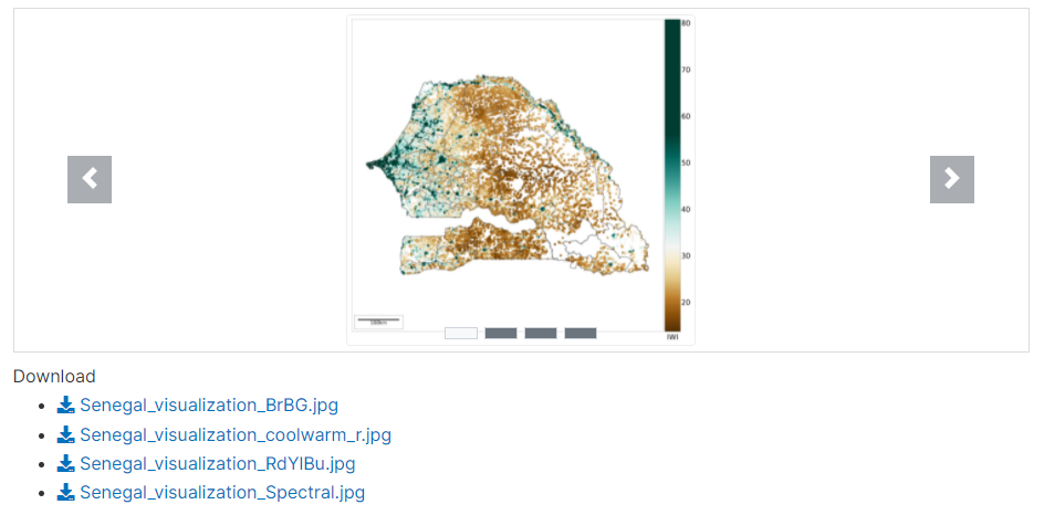
# Displaying a slide show of previews
@@@
# Adding an indicator / time series

Indicators are summary (or "aggregated") measures related to key issues or phenomena, derived from a series of observed facts. Indicators form time series when provided with a temporal ordering, i.e. when their values are provided with an annual, quarterly, monthly, daily, or other time reference. In the context of this Guide, we consider as time series all indicators provided with an associated time, whether this time represents a regular, continuous series or not. For example, the indicators provided by the Demographic and Health Surveys (DHS) StatCompiler (opens new window), which are only available for the years when DHS are conducted in countries (which for some countries can be a single year), would be considered as "time series".
Time series are often contained in multi-indicators databases, like the World Bank's World Development Indicators - WDI (opens new window), whose on-line version contains 1,430 indicators (as of 2021). To document not only the series but also the databases they belong to, we propose two metadata schemas: one to document series/indicators, and one to document databases. In the NADA application, a series can be documented and published without an associated database, but information on a database will only be published when associated with a series. The information on a database is thus treated as an "attachment" to the information on a series.
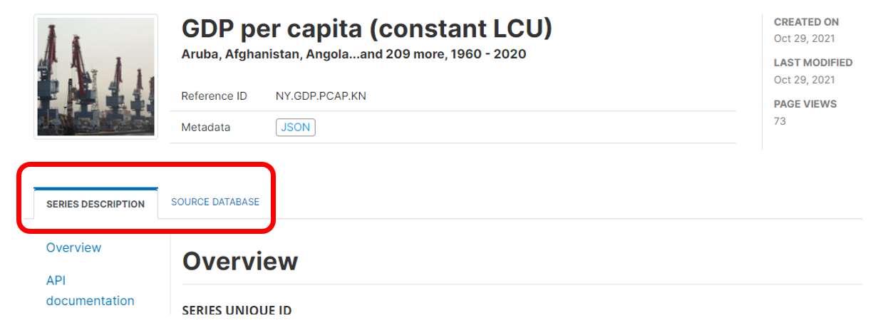
In a NADA catalog, a SERIES DESCRIPTION tab will display all metadata related to the series. The (optional) SOURCE DATABASE tab will display the metadata related to the database, is any. The database information is displayed for information; it is not indexed by the NADA catalog.
Metadata schemas
For documenting indicators/time series and their databases, NADA makes use of two metadata schemas developed by the World Bank Development Data Group: one for documenting the time series/indicators, the other one to document the database (if any) they belong to.
The documentation of the time series metadata schema is available at https://ihsn.github.io/nada-api-redoc/catalog-admin/#operation/createTimeSeries (opens new window). The documentation of the database metadata schema is available at https://ihsn.github.io/nada-api-redoc/catalog-admin/#operation/createTimeseriesDB (opens new window). A Schema Guide is also available, which provides more detailed information on the structure, content, and use of the metadata standards and schemas.
# Loading metadata (web interface)
This option is currently not available. It will be added in a future version of NADA.
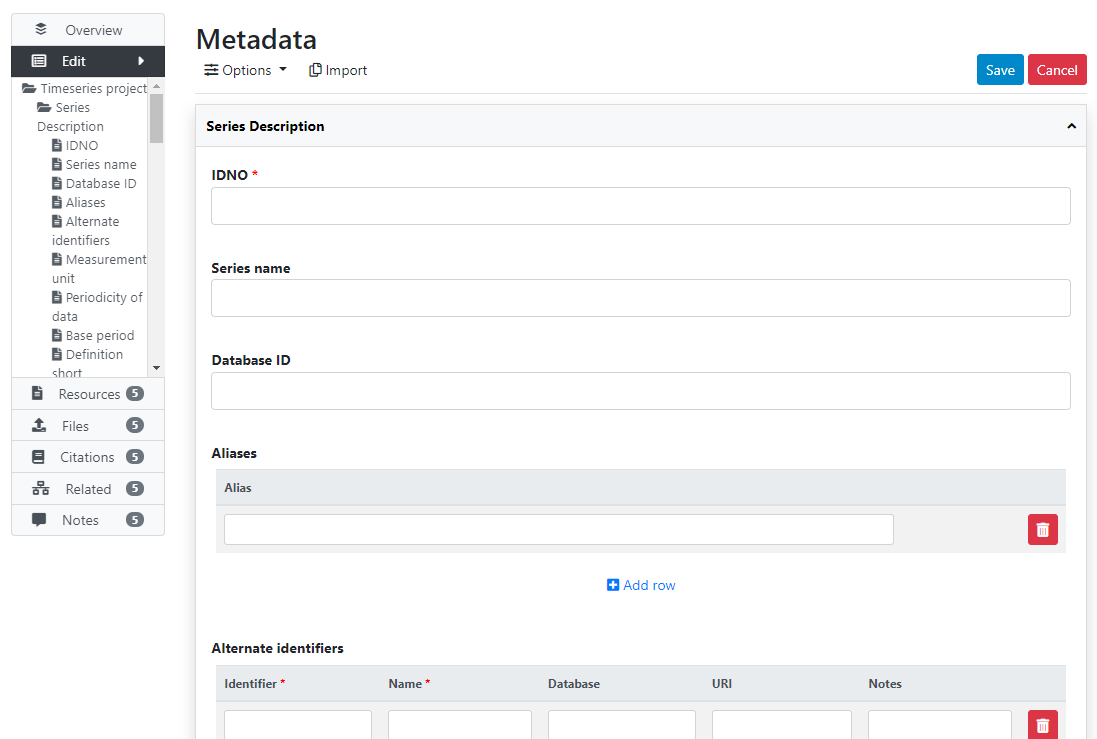
# From scratch (web interface)

# Loading metadata (API)
This option is currently not available. It will be added in a future version of NADA.
# From scratch (API)
You can generate the metadata using R or Python, then publish it using the NADA API and the NADAR package or PyNADA library.
Use Case 007
# Making the data accessible via API
@@@@ Data can be published and made accessible via API. See section ...
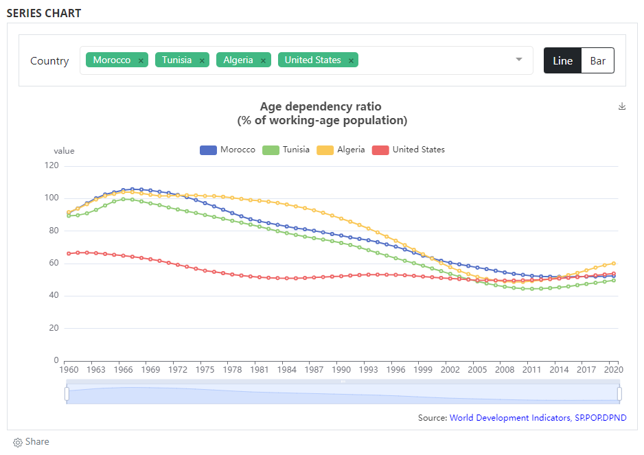
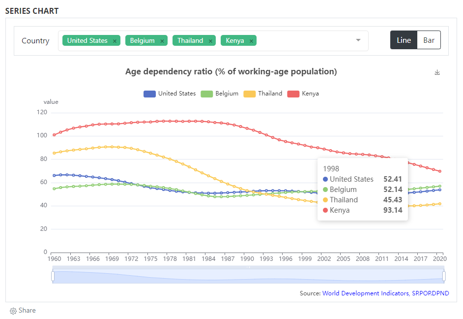
# Adding data visualizations
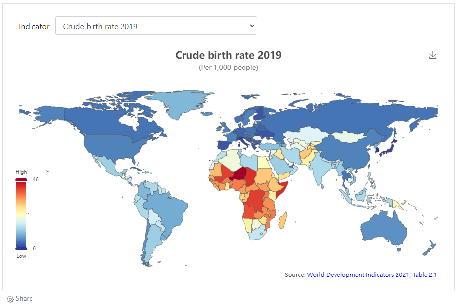
When data are made accessible via API (or when the dataset is small enough to be embedded in a visualization script), you may add interactive visualizations (charts, maps) in the series' metadata page. The visualizations are generated using external charting or mapping tools, so there is considerable flexibility in the type of visualizations you can embed in a NADA page. The example below provides a very simple example (line chart) developed using eCharts, an open source JavaScript library developed by Baidu and published by the Apache Foundation.
Adding visualizations is done by using widgets. See section ...
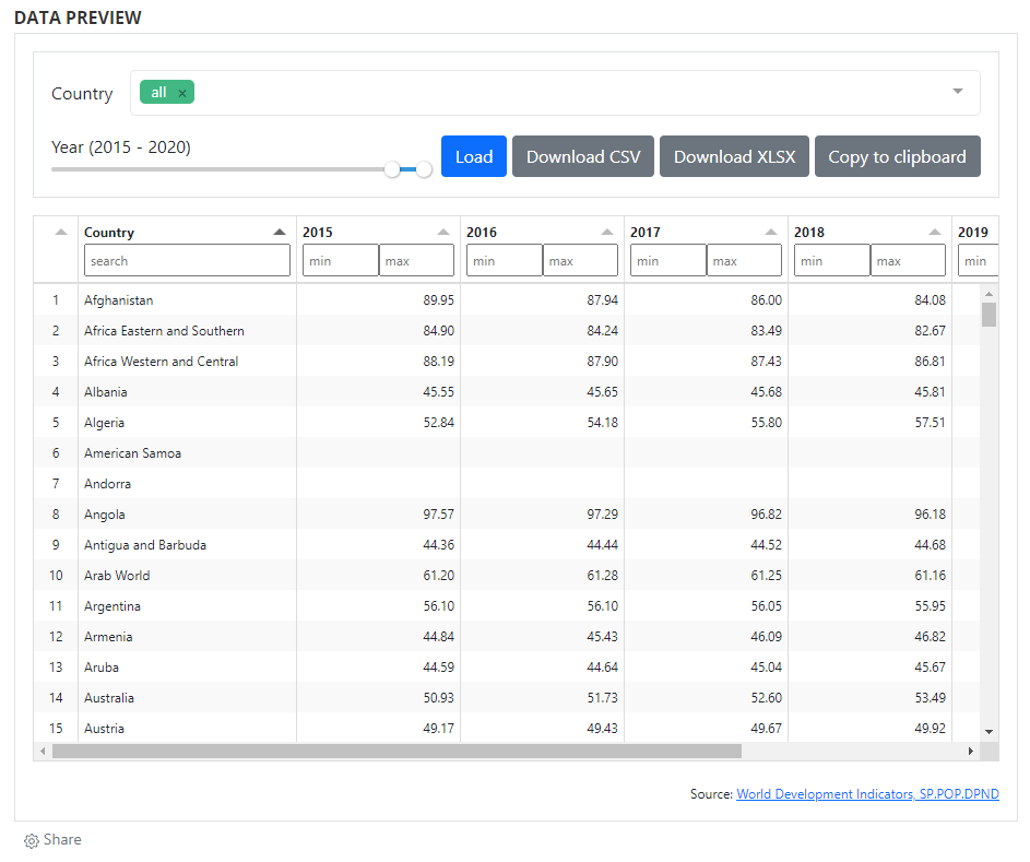
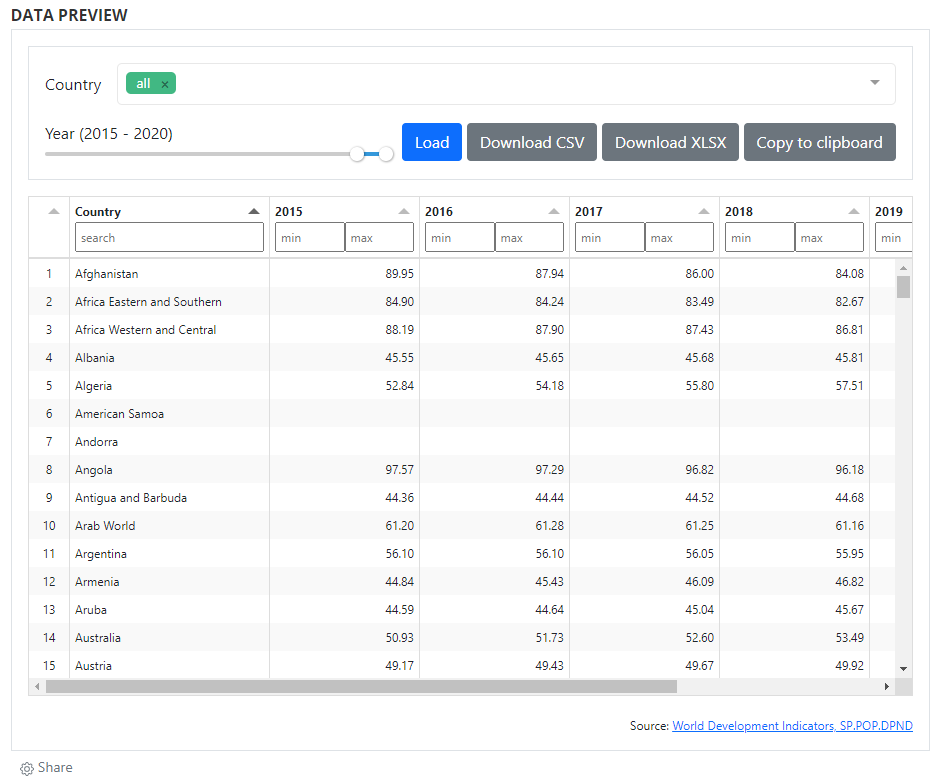
# Adding a data preview
When data are made accessible via API, they can also be displayed and made searchable in a data (pre)view grid. As for data visualizations, this option makes use of external tools and of the widget solution, to provide maximum flexibility to catalog administrators. Multiple open source JavaScript grid applications are availble, as well as commercial ones. The example below makes use of the ... library. For information on how to implement widgets, see section ...
# Adding a table

Metadata schema
For documenting tables, NADA makes use of a metadata schema developed by the World Bank Development Data Group.
The documentation of the table metadata schema is available at https://ihsn.github.io/nada-api-redoc/catalog-admin/#tag/Tables (opens new window). A Schema Guide is also available, which provides more detailed information on the structure, content, and use of the metadata standards and schemas.
# Loading metadata (web interface)
This option is currently not available. It will be added in a future version of NADA.
# From scratch (web interface)
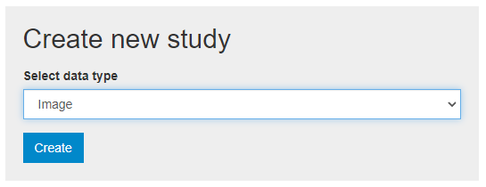
You can create, document, and publish a table using the metadata editor embedded in NADA. To do so, login as administrator, then in the login sub-menu, select Site administration. In the Studies menu, select Manage studies / Central Data Catalog (or another collection), then click on Add study. In the Create new study box, select Table.

Click on Metadata. In the metadata editor form, enter all available information to describe the table, then click on the Save button.
What has been done so far is generating and publishing the table description in the catalog. We have not provided any link to the table, or uploaded the table file to the web server (e.g. as an XLS file, or as a PDF file). Click Add new resource and provide information on the type of resource (in this case a table). Click Submit. @@@@@@@ provide URL or filename/path.
Now the table metadata and the link to the table are both provided. But the entry is still in draft mode (i.e. only visible to administrators); to make it visible to users, change its staus to "Published".
# Loading metadata (API)
This option is currently not available. It will be added in a future version of NADA.
# From scratch (API)
You can generate the metadata using R or Python, then publish it using the NADA API and the NADAR package or PyNADA library.
We provide here an example of R and Python scripts in which a collection of tables ("Country profiles") from the World Bank's World Development Indicators (WDI) are published and publish in a NADA catalog. These tables are published by the World Bank and made available in CSV, XLS and PDF formats. See "COUNTRY PROFILES" at http://wdi.worldbank.org/table (opens new window). The table is available separately for the world and for geographic regions, country groups (income level, etc), and country. The same metadata apply to all, except for the country tables. We therefore generate the metadata once, and use a function to publish all tables in a loop. In this example, we only publish tables for world, WB operations geographic regions, and countries of South Asia. This will result in publishing 15 tables. We could provide the list of all countries to the loop to publish 200+ tables. The example shows the advantage that R or Python (and the NADA API) provide for automating data documentation and publishing tasks.
When documenting a table using R or Python, the table metadata must be structured using a schema described in https://ihsn.github.io/nada-api-redoc/catalog-admin/#tag/Tables (opens new window).
# Making the data accessible via API
@@@@ Content of table can be published and made accessible via API. See section ...
# Adding data visualizations
@@@
# Adding a data preview
@@@
# Adding a document

Metadata standard: Dublin Core
For documents, NADA makes use of the Dublin Core metadata standard, augmented with a few elements inspired by the MARC21 standard.
The documentation of the Dublin Core metadata standard (as implemented in NADA for documenting publications) is available at https://ihsn.github.io/nada-api-redoc/catalog-admin/#tag/Documents (opens new window). A Schema Guide is also available, which provides more detailed information on the structure, content, and use of the metadata standards and schemas.
In the examples below, we will show different ways to upload a document taken from the World Bank website:

# Loading metadata (web interface)
This option is currently not available. It will be added in a future version of NADA.
# From scratch (web interface)
Login as administrator, then in the login sub-menu, select Site administration

In the Studies menu, select Manage studies / Central Data Catalog

Click on Add study

In Create new study, select Document
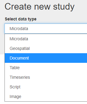
Click on Metadata.

Enter some information in the form, then click on the Save button.
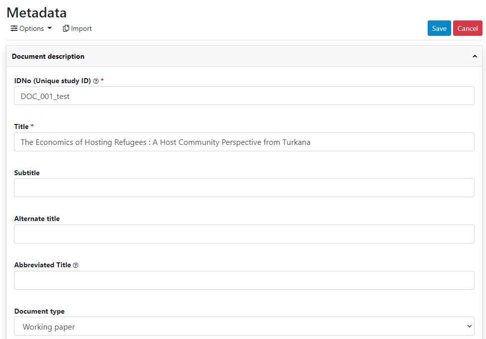
Go back to the entry page (press the "back" button of your browser).
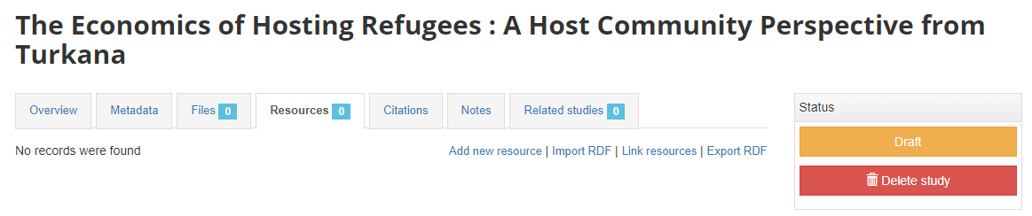
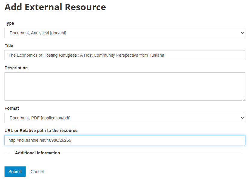
What has been done so far is generating and publishing the document description on the catalog. We have not provided any link to the document. One option would be to upload the PDF to your web server and make the document available from your website. In this case however, we want to provide a link to an external server. Click Add new resource and provide information on the type of resource you are providing a link to (in this case an analytical document), the resource title (in this case it will be the title of the document, but in some cases, you may want to attach multiple files to a document, e.g., an annex containing the tables in Excel format, etc.) Provide a URL to the site you want to link to (the alternative would be to provide the path and filename of the PDF file, for upload to your server). Click Submit.
Now the document metadata and the link to the resource are both provided. But the entry is still in draft mode (i.e. only visible to administrators).
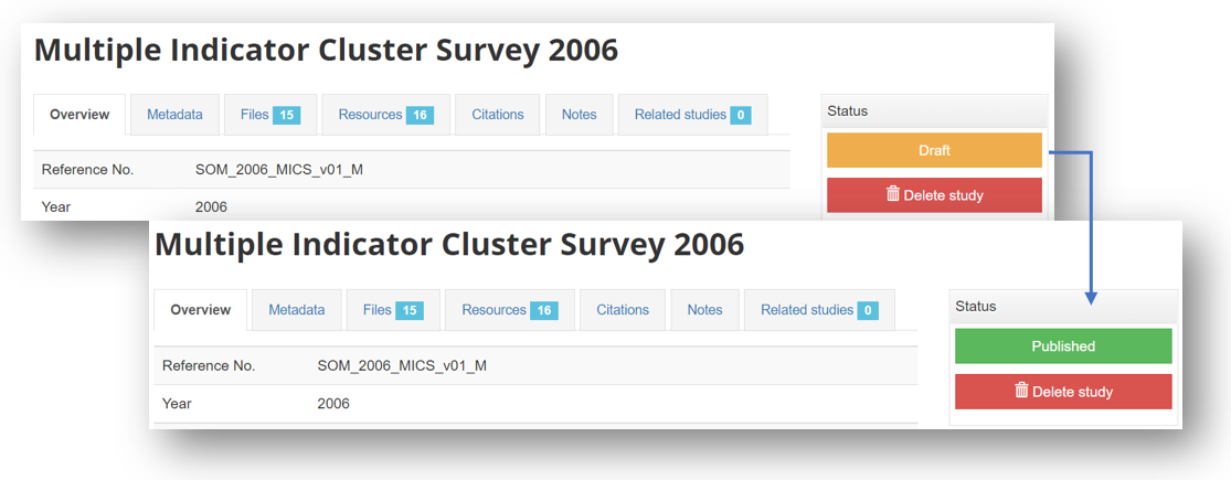
The last step will be to upload a thumbnail (optional), and to make this entry visible in your catalog by changing its Status from "Draft" to "Published". For a document, a screenshot of the cover page is the recommended thumbnail.


The entry is now visible to visitors of your catalog and in the Dashboard of the Site administration interface (where you can unpublish or delete it).
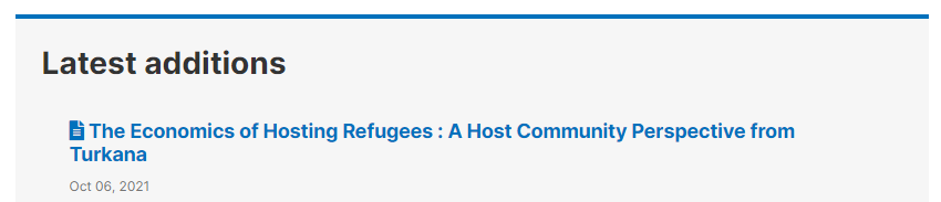
The study listing page in the user interface, with no thumbnail:
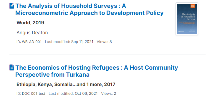
The study listing page in the user interface, with thumbnail:

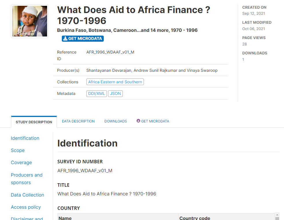
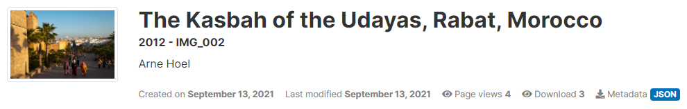
The header of the entry page, with no thumbnail:
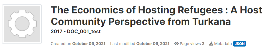
The header of the entry page, with a thumbnail:

# Loading metadata (API)
This option is currently not available. It will be added in a future version of NADA.
# From scratch (API)
You can generate the metadata using R or Python, then publish it using the NADA API and the NADAR package or PyNADA library.
An example of R and Python scripts was provided in section "Getting Started -- Publishing a document". That example is available in the NADA GitHub repository as Use Case 001.
We provide here another example, where a list of documents with their core metadata is available as a CSV file. A script (written in R or in Python) reads the file, maps the columns of the file to the schema elements, and publishes the documents in NADA. This example corresponds to Use Case 002 in the NADA GitHub repository.
# Enabling a PDF document viewer
@@@@ iFrame - Show document in NADA page
# Adding an image

Metadata standards: IPTC and Dublin Core
For documenting images, NADA offers two options: the IPTC metadata standard, or the Dublin Core metadata standard.
The documentation of the image metadata schema is available at https://ihsn.github.io/nada-api-redoc/catalog-admin/#tag/Images (opens new window). A Schema Guide is also available, which provides more detailed information on the structure, content, and use of the metadata standards and schemas.
There is currently no option to upload a metadata file (this option will be implemented in future versions of NADA). The available options are to create the metadata in the NADA web interface or programatically using R or Python.
# Loading metadata (web interface)
This option is currently not available. It will be added in a future version of NADA.
# From scratch (web interface)
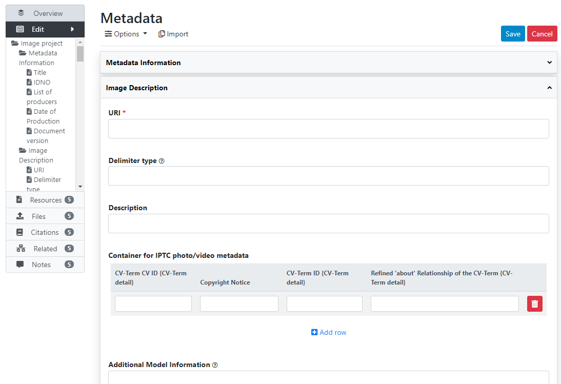
# Loading metadata (API)
This option is currently not available. It will be added in a future version of NADA.
# From scratch (API)
You can generate the metadata using R or Python, then publish it using the NADA API and the NADAR package or PyNADA library.
The API advantage: face detection, labels, ...
# Adding a video

Metadata standards: Dublin Core and schema.org
For documenting videos, NADA uses the Dublin Core metadata standard augmented with some elements from the videoObject from schema.org (opens new window).
The documentation of the video metadata schema is available at https://ihsn.github.io/nada-api-redoc/catalog-admin/#tag/Videos (opens new window). A Schema Guide is also available, which provides more detailed information on the structure, content, and use of the metadata standards and schemas.
# Loading metadata (web interface)
This option is currently not available. It will be added in a future version of NADA.
# From scratch (web interface)
@@@
# Loading metadata (API)
This option is currently not available. It will be added in a future version of NADA.
# From scratch (API)
You can generate the metadata using R or Python, then publish it using the NADA API and the NADAR package or PyNADA library.
# Adding scripts

Documenting, cataloguing and disseminating data has the potential to increase the volume and diversity of data analysis. There is also much value in documenting, cataloguing and disseminating data processing and analysis scripts. There are multiple reasons to include reproducibility, replicability, and auditability of data analytics as a component of a data dissemination system. They include:
- Improve the quality of research and analytical work. Public scrutiny enables contestability and independent quality control; it is a strong incentive for additional rigor.
- Allow the re-purposing or expansion of analytical work by the research community, thereby increasing its relevance, utility and value of both the data and of the analytical work that makes use of them.
- Protect the reputation and credibility of the analysis.
- Provide students and researchers with useful training and reference materials on socio-economic development analysis.
- Satisfy a requirement imposed by peer reviewed journals or financial sponsors of research.
Technological solutions such as GitHub, Jupyter Notebooks and Jupiter Lab have been developed to facilitate the preservation, versioning, and sharing of code, and to enable collaborative work around data analysis. And recommendations and style guides have been produced to foster usability, adaptability, and reproducibility of code. But these solutions do not fully address the issue of discoverability of data analysis scripts, which requires better documentation and cataloguing solutions. We therefore propose --as a complement to existing solutions-- a metadata schema to document data analysis projects and the related scripts. The production of structured metadata will contribute not only to discoverability, but also to the reproducibility, replicability, and auditability of data analytics.
Metadata schema
For documenting scripts/research projects, NADA uses a metadata schema developed by the World Bank Development Data Group.
The documentation of the script metadata schema is available at https://ihsn.github.io/nada-api-redoc/catalog-admin/#tag/Scripts (opens new window). A Schema Guide is also available, which provides more detailed information on the structure, content, and use of the metadata standards and schemas.
# Loading metadata (web interface)
This option is currently not available. It will be added in a future version of NADA.
# From scratch (web interface)
You have the possibility to create a new script entry in the NADA administrator web interface, using the embedded metadata editor. A script entry is used to document and publish all scripts related to one same data processing and/or ananlysis project that involves scripts written in any programming language (R, Python, Stata, SPSS, SAS, other, or a combination of them). The objective of documenting and publishing scripts is to make research and analysis fully transparent, reproducible, and replicable. Ideally, the data that serve as input the the scripts, and the publications that are the output of the analysis, will also be documented and published in the catalog (as microdata, indicators, documents, tables, or other).
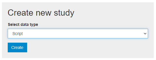
To document a research project (scripts) from scratch using the web interface, select "Add study" in the dashboard page, then select the option script in the Create new study box. Then click Create.
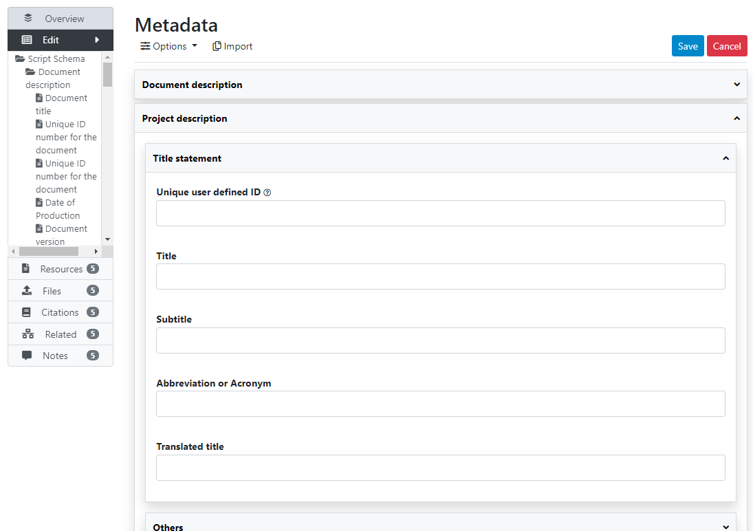
The Overview tab of a new, empty entry will be displayed. Click on the Metadata tab. The metadata editor embedded in NADA will be displayed, providing a form compliant with the NADA metadata schema for documenting data processing and analysis projects. After filling out the fields with as much detail as possible, click on Save.
Once you have entered and saved metadata, proceed as explained in previous section to upload files, select options, add a thumbnail, and publish your metadata. To add external resources, use the Add resource in the External resources page.
# Loading metadata (API)
This option is currently not available. It will be added in a future version of NADA.
# From scratch (API)
You can generate the metadata using R or Python, then publish it using the NADA API and the NADAR package or PyNADA library.
# Featuring an entry
@@@
# Deleting an entry
# Using the administrator interface
# Using the API
Deleting an entry (of any type except external resource) from a catalog only requires knowing the unique identifier of the entry in the catalog. The entry can then be deleted using NADAR (for R users) or PyNADA (for Python users), after providing an API authentication key and the URL of the catalog, as follows (assuming the entry to be deleted has an ID = ABC123):
In R:
library(nadar)

my_keys <- read.csv("C:/CONFIDENTIAL/my_keys.csv", header=F, stringsAsFactors=F)
set_api_key(my_keys[5,1])  # Assuming the key is in cell A5
set_api_url("http://nada-demo.ihsn.org/index.php/api/")

catalog_delete(idno = "ABC123")
In Python:
import pynada as nada

my_keys = pd.read_csv("confidential/my_keys.csv", header=None)
nada.set_api_key(my_keys.iat[4, 0])  # Assuming the key is in cell A5
nada.set_api_url('http://nada-demo.ihsn.org/index.php/api/')

nada.catalog_delete(idno = "ABC123")
# Deleting external resources
# Using the administrator interface
# Using the API
In R:
library(nadar)

my_keys <- read.csv("C:/CONFIDENTIAL/my_keys.csv", header=F, stringsAsFactors=F)
set_api_key(my_keys[5,1])  # Assuming the key is in cell A5
set_api_url("http://nada-demo.ihsn.org/index.php/api/")

@@@@@@@
In Python:
import pynada as nada

my_keys = pd.read_csv("confidential/my_keys.csv", header=None)
nada.set_api_key(my_keys.iat[4, 0])  # Assuming the key is in cell A5
nada.set_api_url('http://nada-demo.ihsn.org/index.php/api/')

@@@@@@@@
# Replacing an entry
# Using the administrator interface
# Using the API
# Editing an entry
Risk of discrepancy
# Using the administrator interface
# Using the API
Powerful automation options. Can programmatically change any specific piece of metadata, for one or multiple entries.
See the NADAR or PyNADA documentation.
# Publishing/unpublishing
# Using the administrator interface
In the Manage studies page:


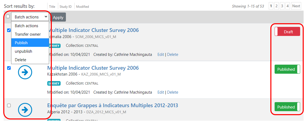
In the study page:
# Using the API
# Making data accessible via API
In addition to providing tools to maintain metadata via API, NADA provides a solution to store and disseminate data via API. In the current version of NADA, this solution applies to indicators/time series and tabular data. It could also be implemented to microdata (this option is not documented here, but will be added in future versions of the documentation).
Making your data accessible via API has multiple advantages:
- Many data users will appreciate such mode of access; all modern data dissemination systems provide an API option.
- By making your data accessible programatically, you provide new opportunities to data users, which will increase the use and value of your data.
- The API can be used internally by your NADA catalog, to create dynamic visualizations, display data, and create on-line data extraction tools.
NADA stores the data and the related data dictionary in a mongoDB database (an open source software). To make use of the data API solution, mongoDB must have been installed on your server. See the Installation Guide for more information.
Publishing data in mongoDB and making them accessible via API is a simple process that consists of:
- Preparing your data: data must be stored in a CSV file (or a zipped CSV file) and organized in a long format. The content of this CSV file will be a "table" in mongoDB.
- The CSV (or zip) file is published in a mongoDB database using the NADAR package (for R users) or the PyNADA library (for Python users). A name will have to be given to the database. A database can contain multiple tables. There is currently no option to publish data to mongoDB using the NADA web interface.
- A data dictionary is created (in R or Python) and published together with the data.
- The data is then accessible via API.
# Formatting and publishing time series data
Time series / indicators will typically come in a format suitable for publishing in the NADA API. The CSV data file must include (i) the series’ unique identifier, (ii) the series features (or dimensions), and (iii) the value.
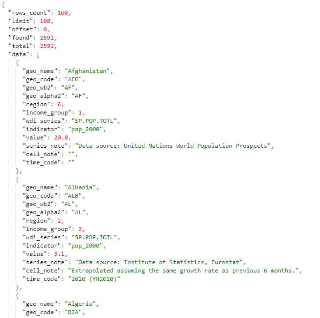
- The identifier will be a string or a numeric variable that provides a unique identifier for the series/indicator. For example, the World Bank’s identifier for the Population, Total series of the World Development Indicators (WDI) database is SP.POP.TOTL. It is SP.POP.TOTL.FE.IN (opens new window) for the female population and SP.POP.TOTL.MA.IN (opens new window) for the male population.
- The features (or dimensions) of the series/indicator are additional qualifiers of the values of the series/indicator. For example, the features for the Population, Total series could be “country_name”, “country_code”, and “Year”. The features are the information that, combined with the series identifier, will provide the necessary information to define what a given value represents.
- The value is the estimate that corresponds to the series and its features.
Example:
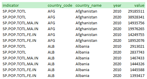
Note that the database could have be organized differently. The WDI database generates separate series for “Population, Total”, “Population, Male”, and “Population, Female”. Another option would have been to create one series “Population” and to provide the sex as a feature:
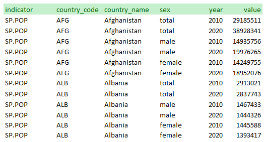
To be published in the NADA data API (as a mongoDB table), the data must first be formatted and saved as a CSV file. The data must be organized as displayed in the examples above, i.e. in a long format (by opposition to a wide format). This means that:
- the data file must have one and only one value per row
- the combination of the series/indicator identifier with the features cannot contain duplicates (in the example above, this means that each combination of series + country_code + country_name + year must be unique in the data file; this will guarantee for example that we would nnot have two different values for the total population of Afghanistan for a same year).
Note that a CSV file may contain more than one series/indicator.
For efficiency reason (reduced file size and speed of data filtering and extraction), it is recommended to store the information in the CSV file as numeric variables whenever possible. In our example, instead of storing the sex feature as a string variable with categories “total”, “male”, and “female”, we could store it as 0 (for total), 1 (for male), and 2 (for female). Also, the country_name variable could be dropped, as the country_code variable provides the necessary information (as long as the user is provided with the country name corresponding to each code). A data dictionary will always be uploaded with the CSV file, which will contain the necessary data dictionnary.

When published in mongoDB, the CSV file will be provided with the following core metadata:
- A unique table identifier (the table refers to a mongoDB table; it corresponds to the dataset being published, which may contain one or multiple time series/indicators).
- The table (dataset) title
- An optional (but recommended) description of the table (dataset).
- A description of the indicator for which values are provided, including a label and a measurement unit.
- A data dictionary containing the variable and value labels for all features (dimensions), except when the value labels are available in a separate lookup file (see section "Using lookup files" below).
Using R
Description of the NADAR function: data_api_create_table( db_id, table_id, metadata, api_key = NULL, api_base_url = NULL ) Arguments db_id (Required) database name table_id (Required) Table name metadata Table metadata
library(nadar)
library(readxl)

# ------------------------------------------------------------------------------
# Set API key (stored in a CSV file; not to be entered in clear) and catalog URL
my_keys <- read.csv("C:/confidential/my_API_keys.csv", header=F, stringsAsFactors=F)
set_api_key(my_keys[2,2])  # Assuming the key is in cell B2
set_api_url("https://nada-demo.ihsn.org./index.php/api/")
set_api_verbose(FALSE)
# ------------------------------------------------------------------------------

tblid = "POP_2010_2020"
csv_data = "C:\test_files\POP_SEX_2010_2020.CSV"

# Generate the table metadata

my_tbl <- list(

  table_id    = tblid,
  title       = "Population by sex, 2010 and 2020, Afghanistan and Albania",
  description = "The table provides population data for two countries, in 2020 and 2020.
	         Source: World Bank, World Development Indicators database, 2021",

  indicator = list(
	list(code   = 10,
             label  = "Population, Total",
             measurement_unit = "Number of persons"),
	list(code   = 11,
	     label  = "Population, Male",
	     measurement_unit = "Number of persons"),
	list(code   = 12,
	     label  = "Population, Female",
	     measurement_unit = "Number of persons")
  ),

  features = list(

    list(feature_name  = "country_code",
         feature_label = "Country",
         code_list = list(list(code="AFG", label="Afghanistan"),
                          list(code="ALB", label="Albania"))),

    list(feature_name  = "sex",
         feature_label = "Sex",
         code_list = list(list(code=0, label="All"),
                          list(code=1, label="Male"),
                          list(code=2, label="Female")))

    list(feature_name  = "year",
         feature_label = "Year")

  )

)

# Publish the CSV file to MongoDB database
publish_table_to_MongoDB(tblid, csv_data, my_tbl)
Using Python
Description of the PyNADA function: @@@
# Same example, in Python
# Formatting and publishing tabular data
The content of statistical tables (cross-tabulations), when it can be converted to a long format, can also be published in the data API. We provide here a simple example. Using R or Python, the format of statistical tables can be reshaped to match the requirements of the NADA data API, saved as CSV, and published in mongoDB. We provide here a simple example.
The source table
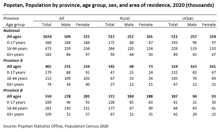
The table contains 108 cells with values. When converted to a long format, we therefore expect to have 108 observations in the resulting CSV file. The indicator is “population”. The features are the province (including the total), the age group (with 4 possible values), the area of residence (with 3 possible values), and the sex (with 3 possible values). The conversion to the long format can be done in Excel, or programmatically (Excel, R, Python, Stata, SPSS, etc. provide tools to reshape tables and to encode variables).
Note: empty/missing values in CSV … Note: do not round
Rule: most detailed and full transparency to users (when they see a value, they need to know what it represents).
Converted to long format

Optimized (encoded strings)

Using R
library(nadar)
library(readxl)

# ------------------------------------------------------------------------------
# Set API key (stored in a CSV file; not to be entered in clear) and catalog URL
my_keys <- read.csv("C:/confidential/my_API_keys.csv", header=F, stringsAsFactors=F)
set_api_key(my_keys[2,2])  # Assuming the key is in cell B2
set_api_url("https://nada-demo.ihsn.org./index.php/api/")
set_api_verbose(FALSE)
# ------------------------------------------------------------------------------

tblid = "POP_AGE_2020"
csv_data = "C:\test_files\POP_AGE_2020.CSV"

# Generate the table metadata

my_tbl <- list(

  table_id    = tblid,
  title       = "Popstan, Population by province, age group, sex, and area of residence, 2020 (thousands)",
  description = "The table provides data on the resident population of Popstan as of June 30, 2020,
                 by province, age group, area of residence, and sex.
                 The data are the results of the population census 2020.",

  indicator = list(list(code   = 1,
                        label  = "Population",
                        measurement_unit = "Thousands of persons")),

  features = list(

    list(feature_name  = "province",
         feature_label = "Province",
         code_list = list(list(code=0, label="All"),
                          list(code=1, label="Province A"),
                          list(code=2, label="Province B"))),

    list(feature_name  = "area",
         feature_label = "Area of residence (urban/rural)",
         code_list = list(list(code=0, label="All"),
                          list(code=1, label="Rural"),
                          list(code=2, label="Urban"))),

    list(feature_name  = "age_group",
         feature_label = "Age group",
         code_list = list(list(code=0,  label="Total"),
                          list(code=1,  label="0 to 17 years"),
                          list(code=2,  label="18 to 64 years"),
                          list(code=3,  label="65 years and above"))),

    list(feature_name  = "sex",
         feature_label = "Sex",
         code_list = list(list(code=0, label="All"),
                          list(code=1, label="Male"),
                          list(code=2, label="Female")))
  )

)

# Publish the CSV file to MongoDB database

publish_table_to_MongoDB(tblid, csv_data, my_tbl)
Example using Python
# Using lookup files
@@@@@ For long lists of value labels (such as detailed, nested geographic codes): instead of long data dictionary, refer to a table in database.
Example: Census data with population total, by state, district, sub-district, town (urban) or village (rural). System with nested codes. Can be thousands of observations. (show table). Not only very long list, also used for multiple tables.
Another example would be a list of occupations, or industries, used in many tables (national or international classifications, which can be long). Many tables can use the same classification.
In such cases, it would be too tedious and inconvenient to produce a data dictionary in R or Python script.
To do that: ...
# Deleting a mongoDB table
@@@ NADAR: data_api_delete_table(db_id, table_id, api_key = NULL, api_base_url = NULL) Arguments: db_id (Required) database name table_id (Required) Table name
# Replacing a mongoDB table
@@@ overwrite = "yes" in NADAR data_api_publish_table( db_id, table_id, table_metadata, csvfile, overwrite = "no", api_key = NULL, api_base_url = NULL )
# Appending to a mongoDB table
@@@ Not yet implemented.
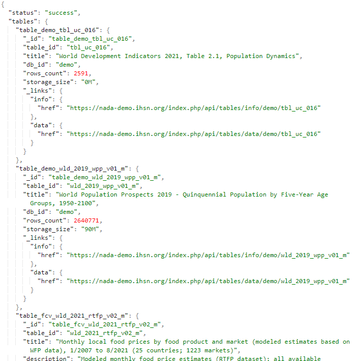
# Listing tables available in mongDB
NADAR: data_api_list_tables(api_key = NULL, api_base_url = NULL)
PyNADA:
Web browser: You can view a list of all tables published in your catalog's mongoDB database by entering the following URL in your browser (after replacing "nada-demo.ihsn.org (opens new window)" with your own catalog URL): https://nada-demo.ihsn.org/index.php/api/tables/list (opens new window). A list of all tables with some summary information on each table will be displayed.
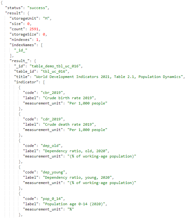
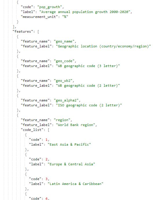
# Retrieving metadata on a table
@@@ https://nada-demo.ihsn.org/index.php/api/tables/info/demo/tbl_uc_016 (opens new window)
# Viewing data in JSON
https://nada-demo.ihsn.org/index.php/api/tables/data/demo/tbl_uc_016 (opens new window)
# Querying the data
@@@
The API will extract data from a database where each cell of each table represents an observation. Some tables contain thousands or even millions of observations. By building and running an API query, you will filter and extract the observations and variables that match your criteria. To build such a filter, you will need (i) the list of variables available in the table, and (ii) the codes used for each variable. For example, if you are interested in extracting ...
Build your query
The information on variables and codes gives you what you need to build your query. The query will always be structured as follows: [base URL][/maximum number of observations (optional)][?][your query][format of data]
The base URL will always be [URL]
The maximum number of observations is an optional parameter. By default, the API will return only the first 400 observations (the rest being available in subsequent pages]. To change this parameter, enter "/" followed by the number.
Your query will start with a "? followed by a list of filters describing the variables and values of interest. This filter can use the operators "AND", "OR", and "!" (not). To select multiple values for a variable, use the "," as a separator or "-" to define a range. For example, to select ...
To list the variables you are interested in, enter "features=" followed by a list of variables separated by commas.
Last, select the format in which you want the data to be returned by the API; the options are "format=JSON" or "format= CSV".
In our example, assume we want ...
# Informing and guiding users
Users will need some instructions to make use of the data API. What to provide? @@@@
# A note on SDMX compatibility
@@@@
# Adding data visualizations
Dynamic visualizations such as charts and maps can be added to a catalog entry page using widgets. The use of widgets is only possible via the API (this cannot be done through the administrator interface). The visualizations are generated outside NADA, for example using a JavaScript library. NADA itself does not provide a tool for creating visualizations; it only provides a convenient solution to embed visualizations in catalog pages. The NADA demo catalog includes such visualizations. See for example:
https://nada-demo.ihsn.org/index.php/catalog/49 (opens new window) (line/bar chart, choropleth map, data preview)
https://nada-demo.ihsn.org/index.php/catalog/87 (opens new window) (choropleth map)
https://nada-demo.ihsn.org/index.php/catalog/97 (opens new window) (age pyramid)
Visualizations can however be applied to any data type, as long as the underlying data are available via an API (the NADA data API, or an external API).
The widgets (zip files) used in the NADA demo catalog are available in the NADA GitHub repository (Use Cases).
# Requirements
A visualization widget can be added to a catalog page in two steps. First, upload a zipped widget source file to a catalog. Second, attach the widget to entry page(s). A zipped widget file contains one [index.html]{.underline} file, and supporting files such as a CSS and a thumbnail image.
In R:
library(nadar)

widgets_create
uuid = widget_uuid,

options = list(
   title = "title of widget",
   thumbnail = "thumbnail.jpg",
   description = "description of widget"
),

zip_file = zip_file

)

widgets_attach(
   idno = dataset_id,
   uuid = widget_uuid
)
In Python:
import pynada as nada

nada.upload_widget(
widget_id = widget_uuid,
title = " title of widget ",
file_path = zip_file,
thumbnail = "thumbnail.JPG",
description = " description of widget "
)

nada.attach_widget(
dataset_id = dataset_id,
widget_id = widget_uuid,
)
With the widget APIs, you can manage widgets and attachments separately. Oftentimes, many entry pages have a common data API and a same type of visualization, in which case a single widget can be used to display different datasets by reading the dataset ID that the widget is attached to as follows:
datasetID = parent.document.getElementsByClassName('study-idno')[0]
Thus, it is advisable to codify key contents of entry pages, such as country names and indicator series, and include the codes in dataset IDs so that a widget can load different data with the codified parameters from data API.
Since a widget is a self-sufficient web application, it is possible to import any JavaScript libraries to visualize data. It is also desirable to utilize a front-end framework (ex. Vue JS) and a CSS framework (ex. Bootstrap JS) to implement a JavaScript widget in a more structured way. The following examples are implemented using open-source Java libraries including jQuery, Vue, Bootstrap, eCharts (chart), Leaflet (map), and Tabulator (grid). Other libraries/frameworks could be used.
# Example 1: eCharts bar/line chart
# Example 2: eCharts map
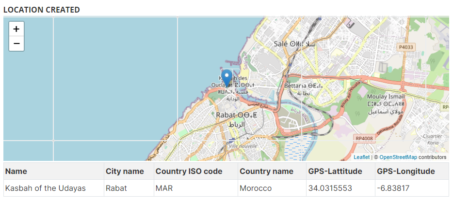
# Example 3: location of image in a OSM map
# Other examples
Demo catalog ; links to GitHub
# Adding a data preview grid
For time series / indicators
The grids are generated outside NADA. In the example below, the grid produced using the open-source W2UI application. Other applications could be used, such as Grid JS, Tabulator, or other (including commercial applications). NADA itself does not provide a tool for generating data grids; it only provides a convenient solution to embed grids in catalog pages.